Coordinates. Graphical representation of functions

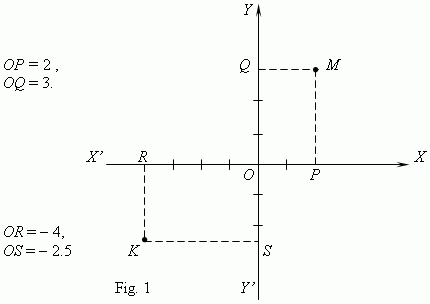
Coordinates. Two mutually perpendicular straight lines XX’ and YY’ ( Fig.1 ) form a coordinate system , called Cartesian coordinates. Straight lines XX’ and YY’ are called axes of coordinates . The axis XX’ is called an x-axis , the axis YY’ – an y-axis . The point O of their intersection is called an origin of coordinates . An arbitrary scale is selected on each axis of coordinates.

Find projections P and Q of a point M to the coordinate axes XX’ and YY’ . The segment OP on the axis XX’ and a number x , measuring its length according to the selected scale, is called an abscissa or x-coordinate of a point M ; the segment OQ on axis YY’ and a number y , measuring its length - an ordinate or y-coordinate of a point M . Values x = OP and y = OQ are called Cartesian coordinates ( or simply – coordinates ) of a point M . They are considered as positive or negative according to the adopted positive and negative directions of coordinate axes. Usually positive abscissas are placed by right on an axis XX’ ; positive ordinates –  by upwards on an axis YY’ . On  Fig.1  we see: a point M has an abscissa x = 2, an ordinate y = 3; a point K has an abscissa x = – 4 , an ordinate y = – 2.5. This can be written as: M ( 2, 3 ), K ( – 4, – 2.5 ).  So, for each point on a plane a pair of numbers (x, y) corresponds, and inversely, for each pair of real numbers (x, y) the one point on a plane corresponds .

Graphical representation of functions.

To represent a functional dependence y = f ( x ) as a graph it is necessary:
1)  to write a set of values of the function and its argument in a table:

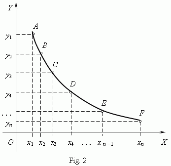
2) To transfer the coordinates of the function points from the table to a coordinate system,
marking according to the selected scale a set of x -coordinates on x -axis and a set of
y -coordinates on y -axis ( Fig.2 ). As a result a set of points A, B, C, . . . , F will be
plotted in our coordinate system.

3)  Joining marked points A, B, C, . . . , F by a smooth curve, we receive a graph of the given
functional dependence.

Such graphical representation of a function permits to visualize a behavior of  the function, but has an insufficient attainable accuracy. It’s possible, that intermediate points, not plotted on a graph, lie far from the drawing smooth curve. Good results also depend essentially on a successful choice of scales. That is why, you should define a graph of a function as a locus , coordinates of points of which M (x, y)  are tied by the given functional dependence.